TensorFlow 到 Caffe2 的 MobileNets 转换器

Linghan Cheung

lhcheung1991@gmail.com

(请在文章底部留下宝贵的评论和建议, Gitment会将留言以issue形式完整保存方便后续查阅)

摘要

Caffe2 是 Facebook 开源的高性能机器学习框架。 Caffe2 旨在模块化，并促进深度学习中的想法和实验的快速原型设计。跟其他主流的机器学习框架相似，Caffe2 支持 C++, Python 等多种编程语言，与此同时，更加强调深度神经网络在移动端上的推断性能（inferrence performance）。与 Google 开源的机器学习框架 TensorFlow 相比，Caffe2 在移动端上的表现足以用惊艳来形容。目前已经有相当多的工程师使用 TensorFlow 进行模型训练和部署，如果为了使用 Caffe2 进行移动端部署而需要重新训练模型，则是一件十分浪费时间和精力的事情。因此，本文尝试对 TensorFlow 模型进行转换，生成对应的 Caffe2 模型，并部署在移动端设备上。本文的主要工作包括：

介绍 MobileNets[1] 模型，并使用 Caffe2 搭建 MobileNets 模型;
介绍 MobileNets 导出器的导出流程（修改网络定义部分便可用于 SqueezeNet 等网络模型的导出），同时指出一些导出过程中可能遇到的坑；
给出模型转换器的效果示例和 MobileNets 在移动端设备上基于 TensorFlow 和 Caffe2 的推断性能比较；
总结

MobileNets

当工程师们在强大的 NVIDIA GPU 支持下进行深度神经网络训练时，很少会考虑到一个参数多、层数深的大模型在移动设备紧巴巴的计算资源上要怎么进行快速的推断。为了获得较高的推断性能，有很多的工作都围绕着如何让模型在移动设备上更高效地推断来进行展开，这些工作大致分为两类，一类是对已经训练好的模型进行压缩，另一类是直接训练较小的模型[1]，MobileNets 模型就是属于第二类的范畴。MobileNets 是由 Google 发布的，专门为了满足移动端和嵌入式设备为设计的小型低延迟网络模型。

MobileNets 提出了两种手段来减少网络推断时的运算量和网络的参数数量：

使用 Depthwise Separable Convolution 这种特殊的卷积层；
使用 2 个超参数——Width Multiplier 和 Resolution Mutiplier 来控制网络的层宽和feature map的大小

标准的卷积操作会对其所在网络的上一层输出进行特征的提取并将多个通道提取出的特征进行融合从而产生新的特征表达，而提取与融合在 Depthwise Separable Convolution 中被分裂成两个层，分别是 depthwise convolution 和 pointwise convolution，其中，depthwise convolution 使用单个的 2D 卷积核对上一层的每个通道进行特征提取，也就是说，上层网络的每个输出通道都对应一个 2D 卷积核，depthwise convolution 运算后将得到相同数目的通道；pointwise convolution 则将 depthwise convolution 的输出通道使用 1 x 1 的 3D 卷积核进行融合，pointwise convolution 层的卷积核个数将决定整个 Depthwise Separable Convolution 的输出通道个数。

具体的 Depthwise Separable Convolution 操作如下图所示[1]：

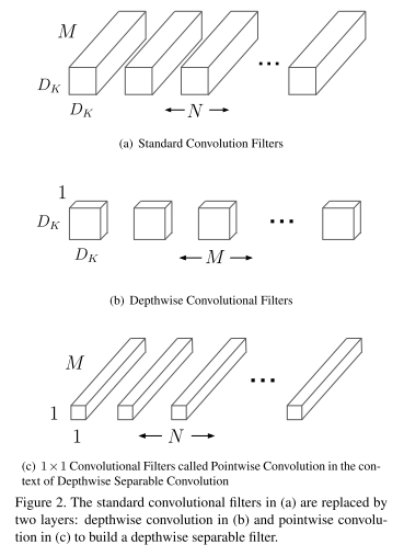
与标准的卷积操作相比，使用 Depthwise Separable Convolution 可以将推断所需的计算量大幅地下降，标准卷积操作的计算代价为：

\[D_{K} \times D_{K} \times M \times N \times D_{F} \times D_{F}\]

Depthwise Separable Convolution 的计算代价为：

\[D_{K} \times D_{K} \times M \times D_{F} \times D_{F} + M \times N \times D_{F} \times D_{F}\]

两者相比的结果如下：

\[\cfrac{D_{K} \times D_{K} \times M \times D_{F} \times D_{F} + M \times N \times D_{F} \times D_{F} }{D_{K} \times D_{K} \times M \times N \times D_{F} \times D_{F}} = \cfrac{1}{N} + \cfrac{1}{D^{2}_{K}}\]

MobileNets 使用 3 x 3 Depthwise Separable Convolution，这样的计算配置可将计算量减少 8 ~ 9 倍。

在上述基础上，MobileNets 使用 Width Multiplier 超参数进一步减少模型的运算量和参数量，其核心的操作是以层为单位，按 Width Multiplier 的比例减少每层的宽度，对于一个使用 Depthwise Separable Convolution 和 Width Multiplier 的网络，其每次卷积的计算量为:

\[D_{K} \times D_{K} \times \alpha M \times D_{F} \times D_{F} + \alpha M \times \alpha N \times D_{F} \times D_{F} \\ where \ \alpha \in (0, 1], \ with \ typical \ settings \ of \ 1, \ 0.75, \ 0.5, \ 0.25\]

此外，MobileNets 还使用 Resolution Mutiplier 超参数来减少网络中的各层通道的大小，加上 Resolution Mutiplier 的 Depthwise Separable Convolution 的计算量大小为：

\[D_{K} \times D_{K} \times \alpha M \times \beta D_{F} \times \beta D_{F} + \alpha M \times \alpha N \times \beta D_{F} \times \beta D_{F} \\ where \ \beta \in (0, 1], \ which \ is \ typically \ set \ implicitly \ so \ that \ the \ input \ resolution \ of \ network \ is \\ \ 224, \ 192, \ 160, \ 128\]

有关 MobileNets 设计思想、准确度与性能试验等内容请参考原文。

下面，我们阐述使用 Caffe2 构建 MobileNets 的过程，如下图为 MobileNets 的标准网络结构图：

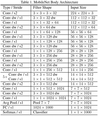
除了第一层卷积层为标准卷积层外，其他的卷积层均为 Depthwise Separable Convolution，每个卷积层之后都会加上一层 BatchNorm 层和 ReLU 层。我们使用 Caffe2 的 caffe2/caffe2/python/brew.py 提供的函数进行搭建。下面代码是 brew.py 提供的常用操作，如 fc 实现全连接层，average_pool 实现平均下采样，spatial_bn 实现 BatchNorm 功能，group_conv 可用于实现 Depthwise Convolution。

_registry = {
		......
        'fc': fc,
        'max_pool': max_pool,
        'average_pool': average_pool,
        'softmax': softmax,
        'spatial_bn': spatial_bn,
        'relu': relu,
        'prelu': prelu,
    	......
        'tanh': tanh,
        'concat': concat,
        'depth_concat': depth_concat,
        'conv': conv,
        'group_conv': group_conv,
        'group_conv_deprecated': group_conv_deprecated,
    	......
    }

下面代码是添加 Depthwise Separable Convolution 的主要操作，有几个需要注意的点：1. depthwise layer 的输入通道数与输出通道数相等；2. group_conv 中的 group 参数等于输入通道数；3. pointwise convolution 的 kernel size 为1。

def addDepthwiseConvAndPointWiseConv(self, filter_in, filter_out, isDownSample):
        _dim_in = int(filter_in * self.width_mult)
        _dim_out = int(filter_out * self.width_mult)
        
        # add depthwise layer
        brew.group_conv(self.model,
                        self.previousBlob, 
                        "depthwise%d" % (self.depthWiseCnt),
                        dim_in=_dim_in,
                        dim_out=_dim_in,
                        kernel=3,
                        stride=(1 if isDownSample is False else 2),
                        pad_t = (1 if isDownSample is False else 0), 
                        pad_r = (1 if isDownSample is False else 1), 
                        pad_b = (1 if isDownSample is False else 1), 
                        pad_l = (1 if isDownSample is False else 0),
                        group=_dim_in,
                        no_bias=True
                       )
        # add bn
        brew.spatial_bn(self.model, ......)
        # add relu
        brew.relu(self.model, ......)
        
        # add conv
        brew.conv(self.model, 
                  "depthwise%d_relu" % (self.depthWiseCnt), 
                  "pointwise%d" % (self.pointWiseCnt), 
                  dim_in=_dim_in, 
                  dim_out=_dim_out, 
                  kernel=1,    # kernel size of pointwise convolution is 1
                  pad=0, 
                  stride=1,
                  no_bias=True)
        # add bn
        brew.spatial_bn(self.model, ......)
        # add relu
        brew.relu(self.model, ......)

网络的构建过程如下，使用 MobileNetBuilder 时需要传入 width_mult 参数，用来控制 MobileNets 的宽度其默认值是 1。使用 workspace.FeedBlob 提前往 workspace 放入数据，可达到 Resolution Mutiplier 参数所起到的控制输入网络图像大小的目的。addDepthwiseConvAndPointWiseConv 中传入 isDownSample 参数用于控制加入的 Depthwise Separable Convolution 是否同时充当下采样层的角色。

raw_data = np.random.randn(1, 3, 160, 160).astype(np.float32)
workspace.FeedBlob("data", raw_data)
mobilenet_model = model_helper.ModelHelper(name="mobilenet")
builder = MobileNetBuilder(mobilenet_model, width_mult=0.5)
builder.addInputDataAndStandConv("data")

builder.addDepthwiseConvAndPointWiseConv(filter_in=32, filter_out=64, isDownSample=False)
builder.addDepthwiseConvAndPointWiseConv(filter_in=64, filter_out=128, isDownSample=True)
builder.addDepthwiseConvAndPointWiseConv(filter_in=128, filter_out=128, isDownSample=False)
builder.addDepthwiseConvAndPointWiseConv(filter_in=128, filter_out=256, isDownSample=True)
builder.addDepthwiseConvAndPointWiseConv(filter_in=256, filter_out=256, isDownSample=False)
builder.addDepthwiseConvAndPointWiseConv(filter_in=256, filter_out=512, isDownSample=True)

for i in range(5):
    builder.addDepthwiseConvAndPointWiseConv(filter_in=512, filter_out=512, isDownSample=False)

builder.addDepthwiseConvAndPointWiseConv(filter_in=512, filter_out=1024, isDownSample=True)
builder.addDepthwiseConvAndPointWiseConv(filter_in=1024, filter_out=1024, isDownSample=False)
builder.addAvgpoolAndFcAndSoftmax()

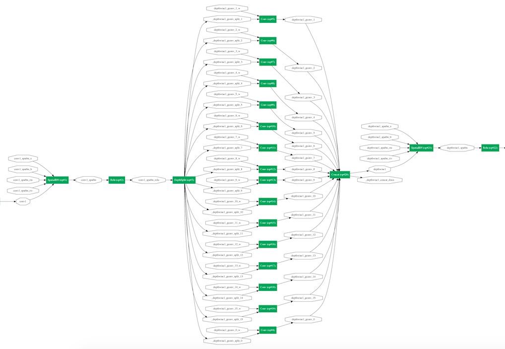
如下所示为第一个 Depthwise Separable Convolution 的网络结构图：

Caffe2 模型导出流程

深度学习框架所导出的模型说到底就是一个包含网络中已经训练得到的参数的文件，所以，本文所介绍的模型转换器的工作原理就是将 TensorFlow 所导出的 MobileNets 的模型参数读取出来，再安放到对应的 Caffe2 的 MobileNets 模型参数中。所以，最关键是弄清楚 Caffe2 的模型是如何被导入的。

Caffe2 和 Caffe 一样，系统内部都使用 Google 的 Protocol Buffers 来处理网络结构的定义和数据的序列化与反序列化。Protocol Buffers 提供了一种类似于 JSON, XML 的结构化定义语言，通过这种语言定义数据的结构，然后使用 Protocol Buffers 编译器产生所需平台的代码，使用这些代码就能很方便对数据进行序列化和反序列化，从而达到跨平台的目的。

Protocol buffers are Google’s language-neutral, platform-neutral, extensible mechanism for serializing structured data – think XML, but smaller, faster, and simpler. You define how you want your data to be structured once, then you can use special generated source code to easily write and read your structured data to and from a variety of data streams and using a variety of languages[2].
// Protocol buffers language
message Person {
  required string name = 1;
  required int32 id = 2;
  optional string email = 3;
}
// generated Java code by protocol buffers compiler
// serializing data with Java
Person john = Person.newBuilder()
    .setId(1234)
    .setName("John Doe")
    .setEmail("jdoe@example.com")
    .build();
output = new FileOutputStream(args[0]);
john.writeTo(output);
// generated C++ code by protocol buffers compiler
// un-serializing data with C++
Person john;
fstream input(argv[1],
    ios::in | ios::binary);
john.ParseFromIstream(&input);
id = john.id();
name = john.name();
email = john.email();

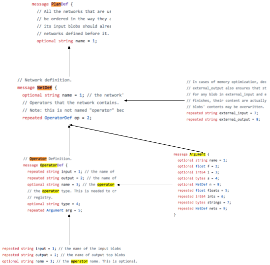
Caffe2 的核心数据，包括网络结构、参数、流经网络中的 tensor 等都是用 Protocol Buffers 进行定义，其定义在 caffe2/caffe2/proto/caffe2.proto 中，各个数据类型之间的包含关系如下图所示，其中，message PlanDef 用于定义网络训练与运行的行为，message NetDef 用于定义网络各层操作的拓扑结构关系、输入输出等属性，message OperatorDef 用于定义各种不同类型的具体操作（如卷积），message Argument 用于定义网络中使用的各种参数。Caffe2 在编译过程中会生成各个平台的代码，这里我们只涉及 C++ 和 Python，通常我们使用 Python 接口定义好网络的结构（此时内存中并没有网络的实例存在），Caffe2 会生成相应的 Protocol Buffers 文件，当我们调用 workspace.RunNetOnce(mobilenet_model.param_init_net)，workspace.CreateNet(mobilenet_model.net) 时，Caffe2 才会根据生成的 Protocol Buffers 文件反序列化出对应的 C++ 实例以保证网络的训练和推断可以由 C++ 提供较高的计算效率。

当使用 caffe2/caffe2/python/model_helper.py 中提供的 ModelHelper 类进行网络构建时，每一个 ModelHelper 实例会默认包含两个 caffe2/caffe2/python/core.py 中定义的 Net 对象实例，而 Net 对象中包含的 self._net = caffe2_pb2.NetDef() 实际上是 caffe2/caffe2/proto/caffe2.proto 中 message NetDef 的实例，也就是说，Net 类是 message NetDef 的 warpper 类，通过调用 print mobilenet_model.net.Proto() 可以看出通过 Python 接口生成的 Protocol Buffers 文件，如下代码所示。

name: "mobilenet"
op {
  input: "data"
  input: "conv1_w"
  output: "conv1"
  name: ""
  type: "Conv"
  arg {
    name: "kernel"
    i: 3
  }
	......
}
......

当使用 p = workspace.Predictor(init_net_serial, predict_net_serial) 初始化推断器（Predictor）时，其所需的 predict_net_serial 文件就包含了网络结构的定义，我们只需使用 Python 定义完网络结构之后，将网络结构的 Protocol Buffers 文件序列化到磁盘中即可 f.write(model.net._net.SerializeToString()) 。而对于包含网络参数的 init_net_serial 文件，则需要将 TensorFlow 中的参数提取出来再转换成 Caffe2 的参数格式。init_net_serial 文件采用与 predict_net_serial 文件相同的格式，由 print mobilenet_model.param_init_net.Proto() 可以看出参数均以 message OperatorDef 形式存放。所以只需使用 caffe2/caffe2/python/core.py 中提供的 CreateOperator 函数创建 OperatorDef 对象，再将参数对应以 message Argument 的形式放入 OperatorDef 对象之中。例如，predict_net_serial 中的第一个 OperatorDef 对象是 MobileNets 的第一个标准卷积层（type: "Conv"），其输入输出为 input: "data"，input: "conv1_w"，output: "conv1"，其中 input: "conv1_w" 就是在 init_net_serial 文件中以 OperatorDef 对象的形式进行数据存储的。

name: "mobilenet_init"
op {
  output: "conv1_w"
  name: ""
  type: "XavierFill"
  arg {
    name: "shape"
    ints: 16
    ints: 3
    ints: 3
    ints: 3
  }
}
op {
  output: "conv1_spatbn_s"
  name: ""
  type: "ConstantFill"
	......
}
......

在 export(INIT_NET, PREDICT_NET, model) 函数中，我们首先将定义网络结构的 model.net._net 进行序列化并写入文件，不过需要注意的是，为了使生成的推断器知道网络最终的输出是什么，我们应该加上网络的输出定义，否则推断器将无法输出最后的预测结果，代码如下所示。我们定义的 MobileNets 的最后一层为网络的输出层，其为最后输出名为 softmax 的 tensor 。

with open(PREDICT_NET, 'wb') as f:
        model.net._net.external_output.extend(["softmax"])
        f.write(model.net._net.SerializeToString())

为了构建存储参数的 init_net_serial 文件，我们需要先定义 NetDef 对象 init_net = caffe2_pb2.NetDef() 。由于 TensorFlow 默认的参数数据顺序为 (H, W, INPUT_CHANEL, OUTPUT_CHANEL)，而 Caffe2 默认的参数数据顺序为 (OUTPUT_CHANEL, INPUT_CHANEL, H, W)，所以从 TensorFlow 中提取的参数需要先做一下维度转换，如下代码所示：

def convert_hwcincout_to_coutcinhw(tensor_in):
    '''
    parameter in tensorflow was organized by H x W x INPUT_CHANEL x OUTPUT_CHANEL
    parameter in caffe2 was organized by OUTPUT_CHANEL x INPUT_CHANEL x H x W
    '''
    pass
    if len(tensor_in.shape) == 1:
        return tensor_in
    ans_np = np.rollaxis(np.rollaxis(tensor_in, 3), 3, start=1)
    # when we use group_conv and channel per group is 1, 
    # we need to reshape tensor to make input channel be 1
    if ans_np.shape[0] == 1:
        return np.rollaxis(ans_np, 1)
    return ans_np

type: "SpatialBN" 的 OperatorDef 对象是 BatchNorm 层，其有 4 个参数，分别是 spatbn_b、spatbn_s、spatbn_rm、spatbn_riv，分别对应 TensorFlow 的 BatchNorm 层的 4 个参数 BatchNorm/beta、BatchNorm/scale、BatchNorm/moving_mean、BatchNorm/moving_variance，需要注意的是，标准的 MobileNets 模型中 BatchNorm 的 Scale 参数为1，所以默认没有 BatchNorm/scale 参数，在进行模型转换时需要给 Caffe2 人工生成 spatbn_s 参数。

创建存放参数的 OperatorDef 对象的核心操作如下代码所示，函数 CreateOperator 的第一个参数为 OperatorDef 对象的类型，我们希望 Caffe2 在初始化推断器时能直接从 init_net_serial 中读取参数值，所以 OperatorDef 对象的类型为 "GivenTensorFill"；第三个参数为参数的名字，其必须与 predict_net_serial 中的参数名字一致；参数 arg 为参数值的列表，描述参数的 shape 和 value。使用 Protocol Buffers 提供的 extend 函数将数据填入 init_net_serial 中，最后使用 init_net.op.extend([core.CreateOperator("ConstantFill", [], ["data"], shape=(1, 3, 160,160))]) 表明输入数据的大小和长宽，类似于 TensorFlow 中 placeholder 一样起到一个占位符的作用。

op = core.CreateOperator("GivenTensorFill", [], [string: name of parameter],arg=[ utils.MakeArgument("shape", tuple: shape of parameter),utils.MakeArgument("values", numpy.ndarray: array of parameter value)
init_net.op.extend([op])

在编写转换器的过程中我们发现，TensorFlow 和 Caffe2 在处理卷积的 padding 时采取了不用的策略。例如，当 stride = 2, kernel = 3 时，TensorFlow 采用 SAME padding，卷积是从通道的左上角开始，而 Caffe2 则会将上下左右都填充1个像素再从左上角开始，修改转换器代码时尤其需要主要这一点，类似于此处的情况，应该使用如下的 padding 方式。

brew.conv(self.model, data, "conv1", dim_in=3, dim_out=32, kernel=3, 
                  stride=2, pad_r=1, pad_b=1, pad_l=0, pad_t=0, no_bias=True)

转换器工作效果 & MobileNets 推断性能对比

我们做了多组图片的推断运算，对比了 TensorFlow 和转换后的 Caffe2 模型在各个中间层的输出结果，数据表明转换后的 Caffe2 模型能在推断时保持小数点后4位的数值精确度，如下图部分数据的对比片段。更多详细的数据对比请运行代码得出。

After average pooling:
tf :
(1, 1, 1, 512)
[ 0.          0.          0.          0.06880768  0.          0.
  0.34500772  0.          0.00759744  0.          0.          0.          0.
  0.02645756  0.          0.          0.          0.          0.          0.
  0.          0.          0.          0.          0.          0.          0.
  0.          0.          0.          0.          0.          0.
  0.00110026  0.          0.          0.          0.00615522  0.01642874
  0.          0.          0.          0.          0.          0.          0.
  0.          0.02483644  0.          0.          0.          0.
  0.03556538  0.          0.          0.06877172  0.          0.
  0.05542048  0.          0.00069364  0.          0.          0.          0.
  0.          0.          0.          0.          0.          0.13392705
  0.          0.          0.          0.          0.          0.
  0.01085833  0.          0.          0.          0.          0.          0.
  0.06680329  0.          0.          0.          0.          0.          0.
  0.          0.          0.          0.          0.          0.
  0.13681063  0.          0.        ]
c2 : 
(1, 512, 1, 1)
[ 0.          0.          0.          0.06880775  0.          0.
  0.34500808  0.          0.00759747  0.          0.          0.          0.
  0.02645758  0.          0.          0.          0.          0.          0.
  0.          0.          0.          0.          0.          0.          0.
  0.          0.          0.          0.          0.          0.
  0.00110034  0.          0.          0.          0.00615523  0.01642861
  0.          0.          0.          0.          0.          0.          0.
  0.          0.02483642  0.          0.          0.          0.
  0.03556541  0.          0.          0.06877175  0.          0.
  0.05542057  0.          0.00069363  0.          0.          0.          0.
  0.          0.          0.          0.          0.          0.13392736
  0.          0.          0.          0.          0.          0.
  0.01085836  0.          0.          0.          0.          0.          0.
  0.06680348  0.          0.          0.          0.          0.          0.
  0.          0.          0.          0.          0.          0.
  0.13681069  0.          0.        ]
---------------------------------
After final convolution:
tf :
(1, 1, 1, 3)
[[[[-1.49511576 -1.07948852  1.84544456]]]]
c2 :
(1, 3, 1, 1)
[[[[-1.49511766]]

  [[-1.07948983]]

  [[ 1.8454473 ]]]]
---------------------------------
After softmax:
tf :
(1, 3)
[[ 0.03252004  0.04927831  0.91820168]]
c2 :
(1, 3, 1, 1)
[[[[ 0.03251991]]

  [[ 0.04927812]]

  [[ 0.91820198]]]]

使用转换的模型生成推断器，输入相同的图片，其输出结果完全一致。

p = workspace.Predictor(init_net_serial, predict_net_serial)
results = p.run([img])
print results
[array([[[[ 0.03251991]],

        [[ 0.04927812]],

        [[ 0.91820198]]]], dtype=float32)]

我们使用 Width Mutipler = 0.5，Resolution Mutipler 使输入的图像为 160 x 160，在多个不同的移动设备上进行推断性能的比较，对比结果如下所示：

	三星 NOTE 3	LG NEXUS 5	魅族 PRO 4	Smartisan Nut
Caffe2	—	70ms	110ms	150ms
TensorFlow	150ms	160ms	250ms

总结

本文 review 了 MobileNets 的相关背景知识，实现 Caffe2 平台上 MobileNets 的搭建，总结了将 TensorFlow 的 MobileNets 导出模型转换成 Caffe2 的方法，并给出数值精确度实验结果和 MobileNets 在两个平台上的推断性能对比结果。下一步工作将围绕提高模型转换器的通用性展开，使之支持更多主流模型的转换功能。

源码

项目源码请移步 https://github.com/lhCheung1991/deeplearning-model-convertor

引用

[1] Howard A G, Zhu M, Chen B, et al. MobileNets: Efficient Convolutional Neural Networks for Mobile Vision Applications[J]. 2017.

[2] Google (2017) Protocol buffers are a language-neutral, platform-neutral extensible mechanism for serializing structured data. https://developers.google.com/protocol-buffers/